Tutorial 1: First Steps with pySimBlocks

Overview

This tutorial introduces the core concepts of pySimBlocks:

• Creating blocks

• Connecting signals

• Running a discrete-time simulation

• Logging and plotting results

By the end of this tutorial, you will be able to build and simulate your own block-based model in Python.

Example File

You can download or view the main example file here:

• main.py

If you have cloned the repository, the full example lives in examples/tutorials/tutorial_1_python/.

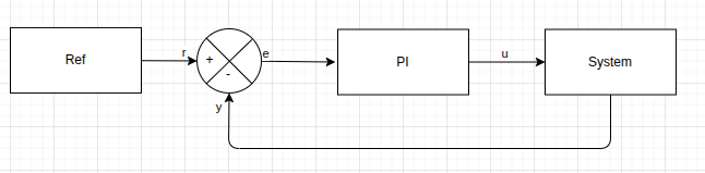
System Description

We build a simple closed-loop control system composed of three elements:

• A step reference

• A PI controller

• A first-order discrete-time linear plant

The plant is a discrete-time first-order linear system defined by:

\[\begin{split} \begin{array}{rcl} x[k+1] &=& a\,x[k] + b\,u[k] \\ y[k] &=& x[k] \end{array} \end{split}\]

The initial state is \(x[0] = 0\).

The PI controller computes a control command from the tracking error \(e[k] = r[k] - y[k]\):

\[ u[k] = K_p\, e[k] + x_i[k] \]

with the integral state evolving as:

\[ x_i[k+1] = x_i[k] + K_i\, e[k]\, dt \]

This integral action removes steady-state error for a step reference.

Complete Example

examples/tutorials/tutorial_1_python/main.py

import matplotlib.pyplot as plt
import numpy as np

from pySimBlocks import Model, SimulationConfig, Simulator
from pySimBlocks.blocks.controllers import Pid
from pySimBlocks.blocks.operators import Sum
from pySimBlocks.blocks.sources import Step
from pySimBlocks.blocks.systems import LinearStateSpace


def main():
    """This example demonstrates how to use the pySimBlocks library to create a 
    simple closed-loop control system with a step reference input, a PI controller, 
    and a linear state-space system.
    """

    A = np.array([[0.9]])
    B = np.array([[0.5]])
    C = np.array([[1.0]])
    x0 = np.zeros((A.shape[0], 1))

    Kp = np.array([[0.5]])
    Ki = np.array([[2.]])

    # -------------------------------------------------------
    # 1. Create the blocks
    # -------------------------------------------------------
    step = Step(
        name="ref",
        value_before=np.array([[0.0]]),
        value_after=np.array([[1.0]]),
        start_time=0.5
    )
    sum = Sum(name="error", signs="+-")
    pid = Pid(name="PID", controller="PI", Kp=Kp, Ki=Ki)
    system = LinearStateSpace(name="system", A=A, B=B, C=C, x0=x0)

    # -------------------------------------------------------
    # 2. Build the model
    # -------------------------------------------------------
    model = Model("test")
    for block in [step, sum, pid, system]:
        model.add_block(block)

    model.connect("ref", "out", "error", "in1")
    model.connect("system", "y", "error", "in2")
    model.connect("error", "out", "PID", "e")
    model.connect("PID", "u", "system", "u")

    # -------------------------------------------------------
    # 3. Create the simulator
    # -------------------------------------------------------
    dt = 0.01 # seconds
    T = 5. # seconds
    sim_cfg = SimulationConfig(dt, T)
    sim = Simulator(model, sim_cfg, verbose=False)

    # -------------------------------------------------------
    # 4. Run the simulation with logging
    # -------------------------------------------------------
    logs = sim.run(logging=[
            "ref.outputs.out",
            "PID.outputs.u",
            "system.outputs.y"
        ]
    )

    # -------------------------------------------------------
    # 5. Extract logged data
    # -------------------------------------------------------
    t = sim.get_data("time")
    u = sim.get_data("PID.outputs.u").squeeze()
    r = sim.get_data("ref.outputs.out").squeeze()
    y = sim.get_data("system.outputs.y").squeeze()

    # -------------------------------------------------------
    # 6. Plot the result
    # -------------------------------------------------------
    fig, axs = plt.subplots(1, 2, sharex=True)
    axs[0].step(t, r, "--r", label="ref", where="post")
    axs[0].step(t, y, "--b", label="output", where="post")
    axs[0].set_xlabel("Time [s]")
    axs[0].set_ylabel("Amplitude")
    axs[0].set_title("Closed-loop response")
    axs[0].grid(True)
    axs[0].legend()

    axs[1].step(t, u, "--b", label="u[k] (pid output)", where="post")
    axs[1].set_xlabel("Time [s]")
    axs[1].set_ylabel("Amplitude")
    axs[1].set_title("PID controller output")
    axs[1].grid(True)
    axs[1].legend()

    plt.show()


if __name__ == "__main__":
    main()

How It Works

The example follows a simple workflow:

1. Blocks are created.

2. Blocks are added to a Model.

3. Signals are connected explicitly.

4. A Simulator executes the model in discrete time.

5. Selected signals are logged and retrieved for plotting.

This reflects the core philosophy of pySimBlocks: explicit block modeling with deterministic discrete-time execution.

About Signal Shapes

All signals in pySimBlocks follow a strict 2D convention:

• Scalars are represented as (1, 1)

• Vectors are (n, 1)

• Matrices are (m, n)

When logging a SISO signal over time, the resulting array has shape (N, 1, 1), where N is the number of simulation steps.

For plotting convenience, the example uses:

y = sim.get_data("system.outputs.y").squeeze()

Try It Yourself

To explore the framework further, try:

• Changing the controller gains Kp and Ki

• Modifying the system dynamics A and B

• Adjusting the time step dt

• Increasing the simulation duration T

Observe how the closed-loop response changes.